
Here is a recap of what we have so far. Our fictional company of interest, WITW, has a FCF of $13 million, with 8 million shares of stock outstanding. Our spreadsheet now has those numbers, and we have entered our guess as to what the future growth of the FCF will be. Now it is time to actually see how much FCF will be available in future years given our growth estimates. Here is the formula to use to determine what the current FCF will be next year:
FCF (next year) = FCF (this year) * (1 + Growth Rate)
So, in our case, FCF (next year) = $13,000,000 * (1 + .07) = $13,910,000
Remember that when talking percentages, in this case 7% growth, to take the percentage and divide by 100 before doing your calculations. Luckily, since we specified Percent as the cell format for the Rate entries, the spreadsheet takes care of this automatically. We are now ready to enter the formula in the spreadsheet, but first let's add a header for Future Value, also known as FV:
Click on cell F8 and enter the following: FV
Formulas in a spreadsheet start with an equals sign (=). This tells the spreadsheet to interpret the rest of the cell as a formula. You can specify normal math operations like multiplication (*), division (/), addition (+), subtraction (-), and more. You can also specify a particular cell by referencing it by its coordinates (for instance B8, or E9). With that in mind, let's enter our formula into the appropriate cell:
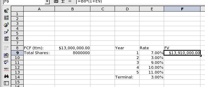
Click on cell F9 and enter the following: =B8*(1+E9)
Pressing Enter after the last operation should reveal something in cell F9. The number is pretty large, so drag the header between columns F and G to resize column F and make it big enough to display the value. After that, your spreadsheet should look something like Figure 6.

Figure 6: Year 1 Future Value (click for full image)
Now that we have the first year, year 2 starts with that result and applies the year 2 growth rate.
Click on cell F10 and enter the following: =F9*(1+E10)
Years 3 through 5 are similar, and we can use a cool little spreadsheet trick to fill those cells. Click in cell F10 and notice there is a little box in the lower-right corner of the cell (see Figure 7).

Figure 7: Cell drag box
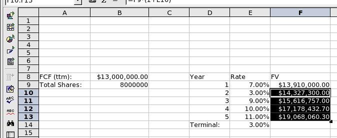
Take the mouse and click in the box, and while holding down the mouse button drag the selection down to cell F13 and release the mouse button. If you were successful, the correct values should have magically appeared in each cell as the spreadsheet adjusted each of the formula values for the appropriate cell. This works because the cells we care about are symmetric. Note that if you had click-dragged cell F9 instead of cell F10, the wrong values would have appeared, since the spreadsheet would have tried to use column B instead of E.
Alright, after that your spreadsheet should look like Figure 8.

Figure 8: Future Value for years 1-5 (click for full image)
We will come back to the FV formula for the terminal growth rate (cell F14) later, since that is different than the other entries. Time to head to the next section where we will take our future estimates and figure out what they are worth today.
Take Me To Part 2 | Take Me To Part 4